Bayesian Regression
Last updated 2025-06-02
Classical Linear Regression
Data
Here’s a simple dataset with a nearly perfect linear relationship between X and Y:
| X | Y | |
|---|---|---|
| 1 | 0.500 | 0.500 |
| 2 | 2.372 | 2.376 |
| 3 | 4.247 | 4.248 |
| 4 | 6.118 | 6.131 |
| 5 | 7.996 | 7.990 |
Linear Regression Model
Using ordinary least squares (OLS) via statsmodels(code not shown), we obtain:
\[Y = 0.0031 + 0.9998X\]
With 95% confidence intervals:
- Intercept: [-0.018, 0.025]
- Slope: [0.996 , 1.004]
This frequentist approach assumes that the only uncertainty lies in the dependent variable Y, and that the residuals are independent, normally distributed, and homoscedastic.
Bayesian Regression (Simple)
Let’s now reframe the same linear model in a Bayesian framework using PyMC.
Model in PyMC
Imports (used throughout this article):
import arviz as az
import pymc as pm
Model definition:
with pm.Model() as linmodel:
  # Priors
  intercept = pm.Normal("intercept", mu=0, sigma=1)
  slope = pm.Normal("slope", mu=1, sigma=1)
  sigma = pm.HalfNormal("sigma", sigma=1)

  # Linear model
  y_pred = pm.Deterministic("model", intercept + slope * (X))

  # Likelihood
  pm.Normal("y_pred", mu=y_pred, sigma=sigma, observed=Y)

  # Inference
  idata = pm.sample(2000, cores=4, nuts_kwargs={"target_accept": 0.95})
ArviZ is used for model diagnostics and summaries.
Sethdi_prob= 0.95 to compute the 95% highest density intervals (HDIs).
Posterior Summary
The estimated regression line is:
\[Y = 0.003 + 1.000X\]
With 95% credible intervals:
- Intercept: [−0.039, 0.038]
- Slope: [0.993, 1.008]
The Bayesian approach treats the model parameters as distributions, not fixed values. The result is a full posterior distribution over all parameters, giving us more than just point estimates – it gives us uncertainty.
Heteroscedasticity in Bayesian
What is Heteroscedasticity?
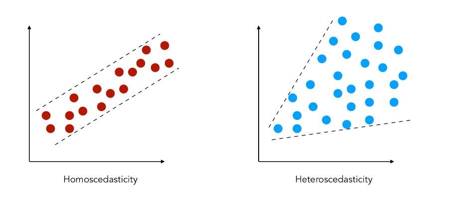
Heteroscedasticity occurs when the variability of the residuals (errors) depends on the value of X. In simpler terms, the spread of Y increases (or decreases) along the range of X. This violates a key assumption of classical OLS regression: constant variance (homoscedasticity).
OLS is not well-equipped for heteroscedastic data. In frequentist settings, one workaround is weighted least squares (WLS) – a method that can get quite nuanced and brittle.
In Bayesian modelling, heteroscedasticity is straightforward to implement.
Data
In this example, each Y value is the average of three repeated measurements (y1, y2, y3), and the standard deviation (sdy) at each point reflects measurement error that increases with X:
| X | y1 | y2 | y3 | Y | sdy | |
|---|---|---|---|---|---|---|
| 1 | 0.500 | 0.549 | 0.549 | 0.550 | 0.549 | 0.001 |
| 2 | 2.372 | 2.614 | 2.616 | 2.615 | 2.615 | 0.001 |
| 3 | 4.251 | 4.667 | 4.691 | 4.680 | 4.680 | 0.010 |
| 4 | 6.134 | 6.751 | 6.735 | 6.736 | 6.741 | 0.007 |
| 5 | 7.998 | 8.791 | 8.784 | 8.813 | 8.796 | 0.013 |
Frequentist WLS (Weighted Least Squares)
Using WLS in statsmodels (code not shown):
\[Y = 0.0057 + 1.0989X\]
With 95% confidence intervals:
- Intercept: [−0.014, 0.025]
- Slope: [1.096, 1.102]
Bayesian Modelling with Heteroscedasticity
All we need to do in PyMC is replace the constant error term sigma with a known, data-derived sdy:
with pm.Model() as hetmodel:
  # Priors
  intercept = pm.Normal("intercept", mu=0, sigma=1)
  slope = pm.Normal("slope", mu=1, sigma=1)

  # Linear model
  y_pred = pm.Deterministic("model", intercept + slope * (X))

  # Likelihood using observed heteroscedastic error
  pm.Normal("y_pred", mu=y_pred, sigma=sdy, observed=Y)

  # inference data
  idata = pm.sample(2000, cores=4, nuts_kwargs={"target_accept": 0.95})
Posterior Summary
Bayesian model estimates:
\[Y = -0.001 + 1.102X\]
With 95% credible intervals:
- Intercept: [−0.003, 0.001]
- Slope: [1.101, 1.103]
Bayesian models allow you to model heteroscedasticity directly and transparently by encoding the varying uncertainty directly in the likelihood – no special workaround needed.
Error-in-variables (Uncertainty in Both X and Y)
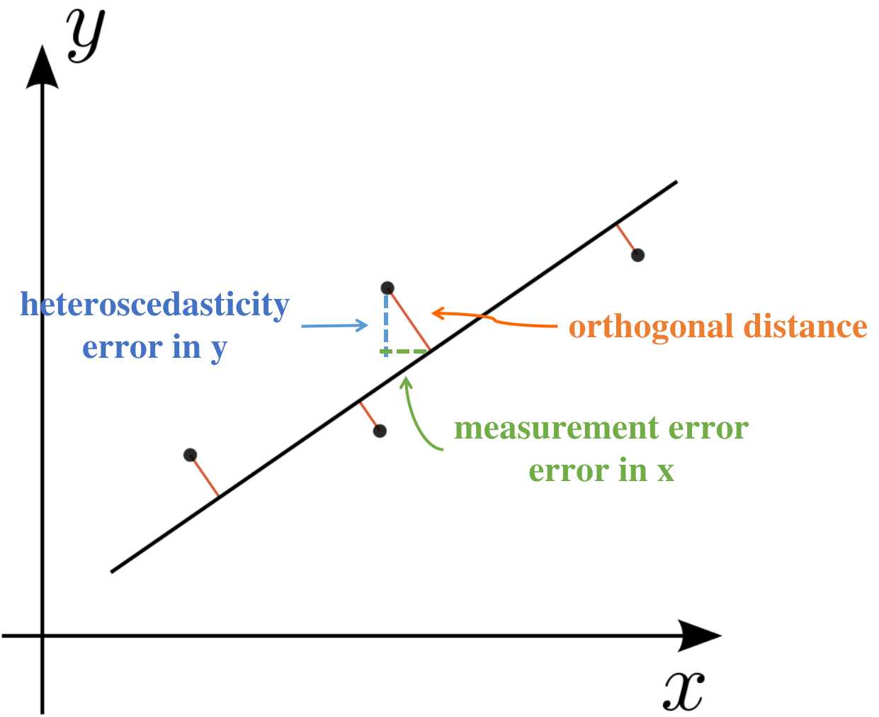
Now let’s address a more challenging scenario: both X and Y have measurement error. This situation frequently arises in real-world experiments.
Why Frequentist Methods Struggle
In the frequentist framework, accounting for measurement error in the independent variable X leads to nontrivial models. One commonly used solution is Deming regression, which assumes known variances in both X and Y and minimizes orthogonal distances rather than vertical residuals.
Even with Deming regression, generalizing to weighted, multivariable, or non-Gaussian cases becomes increasingly messy.
Data
Each X and Y value below is the average of three measurements, with associated standard deviations:
| x1 | x2 | x3 | y1 | y2 | y3 | X | sdx | Y | sdy | |
|---|---|---|---|---|---|---|---|---|---|---|
| 1 | 0.701 | 0.701 | 0.699 | 0.746 | 0.750 | 0.749 | 0.700 | 0.001 | 0.749 | 0.002 |
| 2 | 2.575 | 2.577 | 2.577 | 2.814 | 2.809 | 2.814 | 2.576 | 0.001 | 2.812 | 0.002 |
| 3 | 4.449 | 4.440 | 4.452 | 4.876 | 4.881 | 4.878 | 4.447 | 0.005 | 4.878 | 0.002 |
| 4 | 6.334 | 6.328 | 6.318 | 6.946 | 6.939 | 6.932 | 6.327 | 0.007 | 6.939 | 0.006 |
| 5 | 8.198 | 8.197 | 8.206 | 9.004 | 9.001 | 9.005 | 8.200 | 0.004 | 9.003 | 0.002 |
Weighted Deming Regression (Frequentist)
Estimated model:
\[Y = -0.0227 + 1.1008X\]
95% confidence intervals:
- Intercept: [−0.0268, −0.0186]
- Slope: [1.0995, 1.1020]
Bayesian Error-in-Variables Model
Here’s where Bayesian methods shine. We simply:
- Add a latent variable for the true
Xvalues, modeled with a normal prior centered at the observedX, with standard deviationsdx. - Retain the
sdyinformation in the likelihood, as before.
with pm.Model() as errmodel:
  # Priors
  intercept = pm.Normal("intercept", mu=0, sigma=5)
  slope = pm.Normal("slope", mu=1, sigma=5)

  # Latent variable: true X values
  x_mean = pm.Normal("x_mean", mu=X, sigma=sdx)

  # Linear model
  y_pred = pm.Deterministic("model", intercept + slope * (x_mean))

  # Likelihood with observed error in Y
  pm.Normal("y_pred", mu=y_pred, sigma=sdy, observed=Y)

  # Inference
  idata = pm.sample(2000, cores=4, nuts_kwargs={"target_accept": 0.95})
Posterior Summary
Estimated model:
\[Y = -0.022 + 1.101X\]
95% credible intervals:
- Intercept: [−0.026, −0.018]
- Slope: [1.099, 1.102]
With PyMC, extending your model to account for measurement uncertainty in both X and Y is seamless. This is a powerful advantage over frequentist approaches that require special-case solutions.
Summary
Bayesian regression provides a natural and extensible framework to handle various forms of uncertainty:
- Basic linear regression is straightforward and gives full posterior distributions.
- Heteroscedasticity is easily handled by plugging in known sigma values per observation.
- Error-in-variables becomes a simple matter of introducing latent variables.
Unlike frequentist solutions that often require entirely new techniques or approximations, Bayesian modelling with PyMC evolves incrementally, retaining model transparency and interpretability.